
RAG & Information Retrieval: Understanding the Retrieval Layer
What actually happens between a user's question and the documents supplied to the LLM?
LLMs are remarkably good at generating answers. But generation alone doesn't guarantee that the answer is relevant, up-to-date, or grounded in your organization's data.
Fine-tuning or retraining can help adapt a model to a specific use case, but neither is an ideal solution when the underlying information changes frequently or exists outside the model's training data.
This is where Retrieval-Augmented Generation (RAG) comes in.
RAG
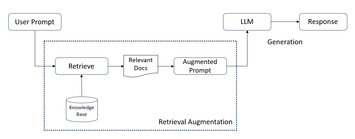
In simple words, give model access to external source of information before generating any response, thereby grounding the response in factual data. From this very sentence, we can see that RAG consists of 2 stages -
Access to secondary information
Response Generation (or Text Generation)
While Transformer-based language models are exceptionally good at text generation, Information Retrieval (IR)—the technology underlying search engines for decades—provides a natural way to retrieve relevant external information before generation.
Hence, RAG architecture became -
Retrieval
Text Retrieval is one of the most critical part of any RAG system. While there are many complexities involved in implementing the same, one of the easiest, fastest implementation came from Information Retrieval (IR) systems.
IR systems have mostly been based on Keyword-Search, i.e. documents are represented using term-based representations and are scored based on the occurrence and importance of query terms. This has been a fast and efficient technique which enabled search engines return matching links/documents based on search queries.
Because the total vocabulary across a corpus can be very large, each document typically contains only a small subset of those terms. As a result, the corresponding vector representation contains mostly zeros and is therefore called a sparse representation. Hence, this approach is commonly referred to as Sparse Retrieval.
Sparse Retrieval
$$Each\ document\ d_i:\ [c_1,c_2,....,c_k]\ -\ vector\ of\ dimension\ k$$
$$k\ =\ total\ unique\ words\ across\ corpus$$
$$c_j\ =\ count\ of\ word\ j\ in\ the\ document\ (simplified\ version)$$
In Sparse retrieval, Each document is saved as a vector representation of word counts. For any incoming user query -
Query is tokenized into words
For each word in the query, a score is computed against each document
Scores for all query words are added as a document score for that query
Documents are then returned as sorted list based on these scores - higher the score, relevant the document
Score Computation
Multiple techniques have been used for computing this 'relevance score', but the 2 main techniques used widely were -
TF-IDF
BM25 (modified TF-IDF)
TF-IDF
Term Frequency (TF) represents frequency (count) of term (word) in the document. Idea: Higher Count --> More Relevant Document
Inverted Document Frequency (IDF) represents inverted count of documents containing the term (word). It is used to give additional importance to rare, meaningful words
Formally defined as -
$$TF(t,d) = 1+log_{10}Count(t,d),\ if\ Count(t,d)\ >\ 0$$
$$TF(t,d) = 0,\ if\ Count(t,d)\ =\ 0$$
$$IDF(t)\ =\ log_{10}(N/DF_t),\ N=total\ docs,\ DF_t=docs\ containing\ word\ t$$
TF will tend to bias towards longer documents, hence, TF is modified as -
$$TF(t,d) = 1+log_{10}(Count(t,d)/total\ words\ in\ doc\ d),\ if\ Count(t,d)\ >\ 0$$
$$Score(q,d)=\sum_{t\in q\cap d} TF_{t,d}\ .\ IDF_{t}$$
Note: A common alternative is to normalize term frequency by document length (as above). The exact TF normalization varies across implementations but the important intuition is that raw term counts can favor longer documents.
Best Matching 25 (BM25)
BM25 can be viewed as an evolution of TF-IDF that introduces tunable controls for 'term-frequency saturation' and 'document-length normalization'. This flexibility has made BM25 one of the most widely used scoring functions for Sparse Retrieval.
Term Frequency Saturation - TF-IDF will uniformly increase the score of documents based on the count of a given keyword in the document. This may or may not be desirable depending upon use case. BM25 introduces a factor, 'k', which can control the effect of term count
Document Length Normalization - TF-IDF either places a full penalty on the length of the document or does not place a penalty at all, based on the TF definition used. BM25 makes it configurable using a factor 'b'.
$$IDF(t) = log_{10}[(N-DF_t+0.5)/(DF_t+0.5)]$$
$$Score(q,d)=\sum_{t\in q\cap d} IDF_{t}\ .\ [(TF_{t,d}.(k+1))\ /\ (TF_{t,d}+k(1-b+b(|d|/avg|d|)))]$$
Here,
|d| = length of document d; Avg|d| = Avg. length of all documents in corpus,
k = commonly between 0.5 to 2; and 0 <= b <= 1
Tuning 'b' - Increase to apply higher normalization like in cases where document sizes are of varying length and longer ones should not dominate.
Tuning 'k' - Increase if term repetition is actually important like legal documents, scientific journals, tech manuals etc.
Indexing
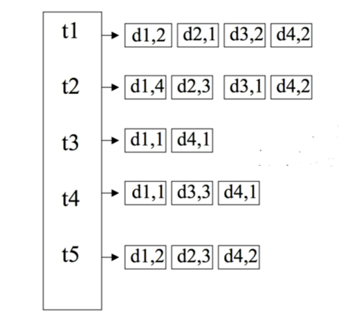
A core data structure behind efficient sparse retrieval is Inverted Index. It maps each term to a postings list containing document IDs and, typically, term-frequency information. This allows the search engine to efficiently retrieve documents containing query terms.
Dense Retrieval
Since Sparse Retrieval is only concerned with occurrence of words, it can only help find documents containing the exact words. Therefore, retrieval accuracy will be low if -
Documents contain synonyms or
Meaning of the document is completely different based on order of words but the words are essentially same as in query
Documents contain few common words but mostly different words but overall context or meaning is similar
Query is specific to rare words or words not present in memory (corpus)
But thanks to Transformer architecture and subsequent explosion of Language Models - big and small, it is now possible to encode the meaning of a document in an embedding (another name for vector representation).
An embedding model is commonly a fine tuned model trained on retrieval objectives, which encodes text into a dense vector representation designed to capture useful semantic information. These vectors are much smaller than a vocabulary-sized sparse representation, hence the term dense vectors. Searching this embedding space is commonly referred to as semantic search.
Here's a quick comparison between Sparse & Dense Retrieval
| Criteria | Sparse Retrieval | Dense Retrieval |
|---|---|---|
| Approach | Lexical Matching | Semantic Matching |
| Unit | Term Based | Embedding Based |
| Strength | Excellent for Exact Terms | Better for Semantic Matching |
| Scoring | BM25/TF-IDF | Cosine Similarity |
| Indexing | Inverted Index | Vector Index |
There are primarily 2 ways of implementing Dense Retrieval -
Cross Encoder
Both query and document are combined into a single input, separated by special tokens, and fed as input to the model. Model is trained to predict a score, representative of the relevance of the document for the given query.
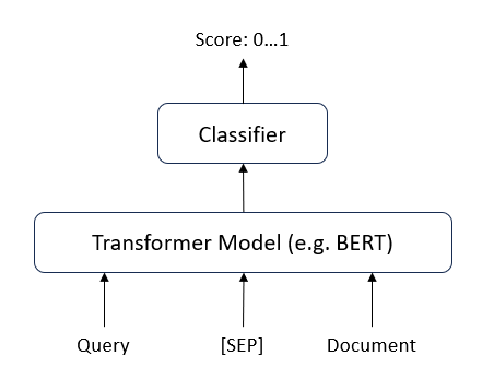
Cross-encoders can model query-document interactions more directly and often provide stronger relevance judgments, but they are substantially more expensive because the query and each candidate document must be processed together
Bi-Encoder
A bi-encoder independently encodes the query and document into vector representations. The model is trained so that relevant query-document pairs have similar representations for e.g. a Siamese Network.
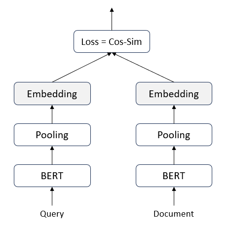
The biggest advantage of Bi-Encoders is that embeddings for all documents can be pre-computed and stored in a vector database (databases specialized for vector storage & retrieval). Whenever a query comes, its embedding is generated using the same model (hence, query & document embeddings will be in same latent space) and is then used to search similar documents using a similarity metric on the embeddings. This makes this approach trade some interaction modeling for superior scalability.
In Production RAG Systems, there are generally 2 stages of dense retrieval -
Retrieval - Bi-Encoders are generally employed for fast retrieval when size of data (documents) is huge. This will help reduce search set to a limited set of relevant documents (commonly called 'candidate set').
Post-Retrieval (Re-Ranking) - Once we get our candidate set, it becomes feasible to run our cross-encoder model to return a more accurate relevance score for each of the candidate documents. Final response is then generated based on the rank of each document, calculated based on cross-encoder's similarity score.
Some common similarity measures used are -
Euclidean Distance - Distance between 2 vectors (L2 Distance)
Dot Product - Sum of element-wise products of two vectors; equivalently, the product of their magnitudes and the cosine of the angle between them
Cosine Similarity (most common) - Measures the angular similarity between two vectors, independent of their magnitude
Hybrid Retrieval
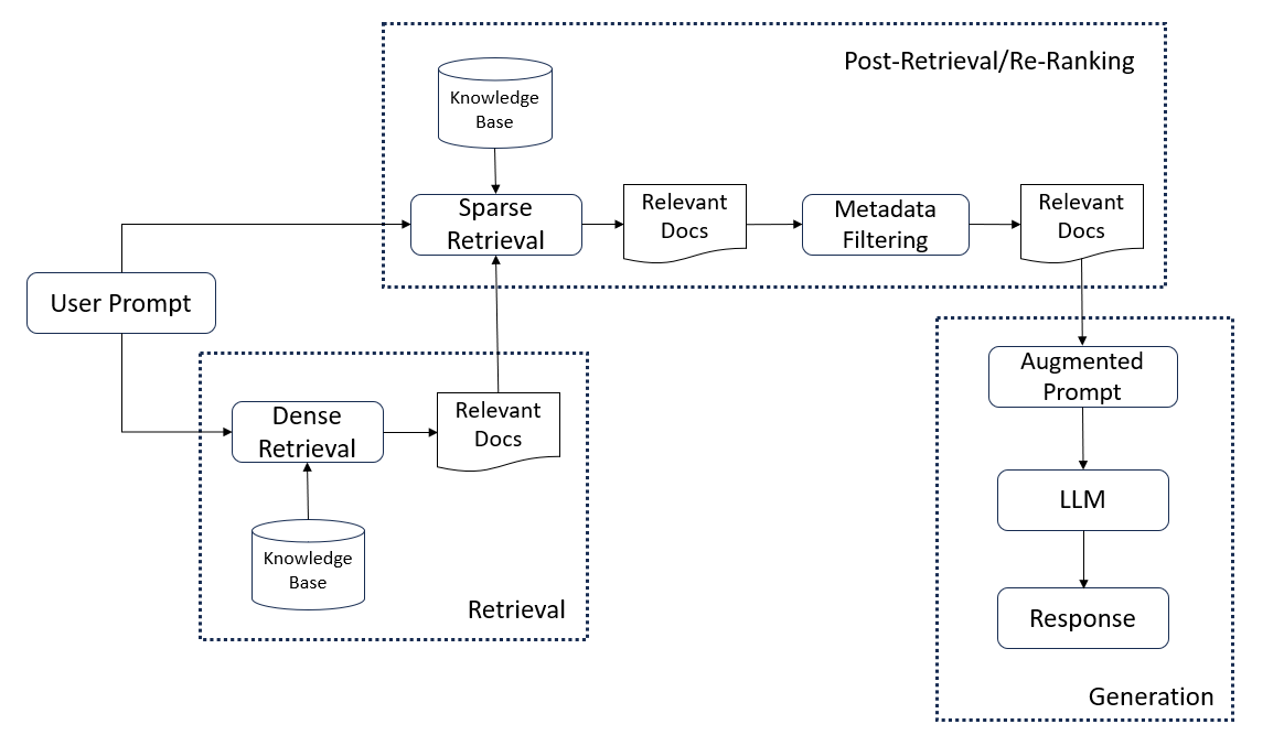
Many Production RAG systems today don't use only one retrieval technique, instead they deploy a Hybrid RAG system where both dense retrieval and sparse retrieval work in tandem. This is then complemented by 'Metadata Filtering' which can be applied alongside retrieval as a business-logic-based constraint—for example, filtering documents by tenant, date, document type, access permissions, or geography.
Production RAG Architecture
Re-Ranking
While above Architecture depicts a Sequential RAG - first Dense, then Sparse and finally Filtering, there are multiple ways of defining this architecture depending upon which leads to highest accuracy -
Sequential
Dense Retrieval as Candidate Selector
Sparse Retrieval for Ranking
Parallel
Dense Retrieval as Ranker 1
Sparse Retrieval as Ranker 2
Combined Ranking Score (Reciprocal Rank Fusion) =
$$Rank = [w_1\ /\ (K+Rank_{Ranker1})]\ +\ [w_2\ /\ (K+Rank_{Ranker2})]$$
$$w_1, w_2 = Weights\ of\ each\ ranker\ (configurable)$$
Metadata Filtering can be used across any design as business-logic based document filter.
Note: To improve final ranking of relevant documents in RAG, sometimes a secondary LLM is also used in Re-Ranking to provide relevance scores.
This concludes the deep dive into the retrieval layer. If you'd like to explore how these concepts come together in a production-grade RAG architecture, check out my next article: Practical Considerations While Designing a Production-Grade RAG System.