Practical Considerations while Designing a Production-Grade RAG System

Note: If you are looking for RAG fundamentals, then please check out my previous article in RAG series - https://ankushagg-ai.hashnode.dev/rag-information-retrieval-understanding-the-retrieval-layer

---

A RAG prototype can be built in a few lines of code. A production-grade RAG system is a very different engineering problem.

Architecture

As discussed in above blog, the architecture of modern RAG systems looks something like this -

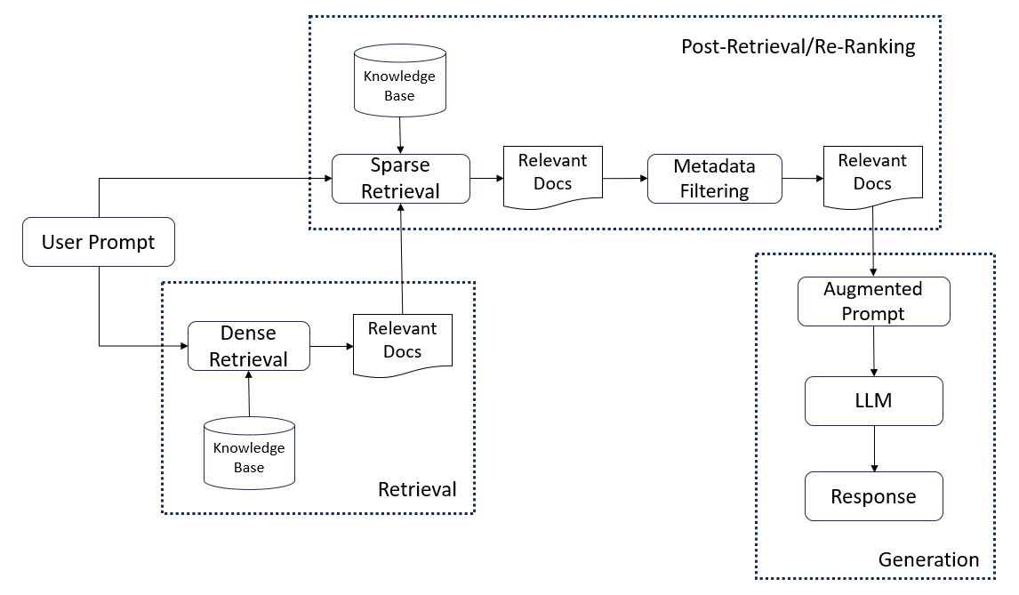
However, many critical nuances are hidden in this simplified diagram, and these details can directly impact system quality, accuracy and performance. To understand these trade-offs, let's look at a much deeper view of Production Grade RAG Systems.

Below is a comprehensive RAG architecture which covers most of the components generally used in Production use cases -

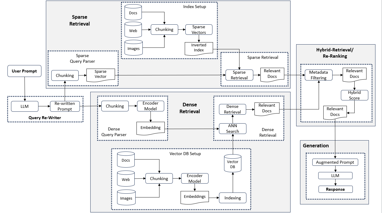
The most critical components in the above architecture which directly impact response relevancy and system performance are -

1. Chunking

2. Indexing

3. Search

Let's understand the challenges and importance of each as well as the techniques used to improve overall system performance.

Note: This article mostly focusses on Dense Retrieval, while Sparse Retrieval is extensively covered in previous article.

Query Re-writing (Optional)

Users interact with LLMs in a very naive/human manner. It can happen that the prompts entered by them can be very verbose and only a small part of the prompt is actually relevant enough to generate the right response.

For e.g. "I went to the garden with my baby and he played a lot with his friends. They played football, played on swings and ran a lot. He is generally fussy about eating. Later we went to the mall and played there as well. Now, he is tired and I don't know what to cook for him quickly".

Such a prompt, if sent for retrieval, will not only cost a lot but will also have higher probability of returning irrelevant results since the response should essentially be about quick, healthy food for the baby and not about games, playing etc.

Therefore, it is sometimes important to use another LLM to first re-write the query before submitting it to the retriever so that things like database search are optimized and high response relevancy is maintained.

Some useful techniques include -

1. Named Entity Recognition (NER) - NER Models can easily identify entities in prompts like person, locations, time, objects etc., which can then be passed as structural signals to the LLM to re-write the prompt. For example, GLINER supports zero-shot NER and can be used when entity extraction is required.

2. Hypothetical Document Embeddings (HYDE) - In this technique, we first generate hypothetical documents which would ideally answer the query. Then we generate its embedding and finally send that embedding to the retriever for finding relevant documents.

Chunking

Chunking is the process of splitting a document into smaller, semantically meaningful units that can be independently embedded and retrieved. It also helps keep each unit within the embedding model's input limits.

Now, if we create too big chunks then there will be too many information within a single chunk. If Embedding Model's context window is small, then a significant part of the chunk can be lost, otherwise the embedding will be too generic since a lot of information will be there in the chunk.

If we create too small chunks, we run the risk of losing surrounding context for each chunk and hence impacting relevance accuracy since few relevant documents might come out as irrelevant because of disjoint chunks.

In short, Chunk Size affects -

1. Retrieval Granularity

2. Embedding Quality

3. Context Preservation

4. Number of retrieved chunks

5. Downstream Context/Token Cost

Hence, right chunking strategy is critical to overall RAG accuracy !

Following are some of the possible chunking strategies which can be selected depending upon the use case -

Fixed Size Chunking

Generally done at a word level or character level, this strategy provides fixed size chunks, even if deriving proper meaning of a text required multiple words within the same chunk.

Tip: Retrieval Quality can be significantly improved with Fixed Size Chunking by adding an overlap of 'n' characters between 2 consecutive chunks, to each chunk. However, optimal overlap depends on the document structure and should be determined through empirical validations.

Recursive Character Text Splitting

This strategy recursively splits text using a hierarchy of separators—for example, paragraphs, newlines and spaces—while attempting to keep related content together. This produces variable-sized chunks and often preserves semantic structure better than blindly splitting at a fixed character count. The only downside is that it can result in too many chunks and also some of the chunks can be small and irrelevant when viewed in isolation.

In most of the practical cases, Fixed Size & Recursive Text Splitting are both used in conjunction. For e.g. texts like heading and follow-up paragraph are first split by recursive character splitting but then headings are merged because of fixed size splitting, thereby, making them more meaningful.

There are also more advanced chunking strategies which help improve accuracy significantly but come with higher cost as well

Semantic Chunking

1. Chunk at sentence level and create vector for each chunk

2. Calculate cosine distance between 2 consecutive chunks

3. If cos-distance > threshold, merge chunks to create bigger chunk

LLM Based Chunking

Use another LLM in the RAG pipeline to create chunks of the source document by including instructions like 'keep concepts together', 'add breaks when new topic starts' etc.

Context-Aware Chunking

Use another LLM to add additional context to every single chunk (e.g. summary text) and re-create the chunk. This strategy is flexible enough to be applied on top of any other previous strategies.

Based on my experience, here is a quick suggestion on when to apply which strategy -

Strategy	Best Suited For
Fixed Size	Simple, Unstructured Text; Cost is critical
Recursive	Structured Documents; Cost is critical
Semantic	Topic-Heavy Documents; Medium Scale
LLM Based	Complex Document Structures; Cost not critical
Context-Aware	When isolated chunks lose meaning; Accuracy is critical

Indexing & Search

Once we have document embeddings (N) and incoming query's embedding (Q), we can find K-Nearest Neighbors for Q using any similarity measure but this will have a high complexity of O(N*D), where

N = number of documents & D = dimension size

In Production Systems, N can run into millions & D can be in thousands, hence, such an exact KNN search approach becomes infeasible.

Since, the way we store our vectors (Indexing) hugely impacts the subsequent search operation (Search), most of the Vector DB providers today provide integrated Indexing & Search functionality.

Inverted Files (IVF)

This solves the problem of 'too many vectors to check' by -

1. Grouping documents into multiple groups (nlist) using clustering algorithms like K-Means and each group's centroid vector is calculated

2. Each group is then organized as Inverted Lists (remember BM25!) labelled by group's centroid vector

3. For given Q, we first run similarity search with all the centroid vectors

4. Then, find most similar documents only from within the groups whose centroid vectors were the closest.

This can dramatically reduce the number of database vectors that need to be compared, trading some recall for lower search cost.

Product Quantization (PQ)

In this approach, original vector is partitioned into 'm' sub-vectors/sub-spaces and a separate codebook is learned for each sub-space independently. Each sub-vector is then represented by the ID of its nearest codeword, significantly reducing the memory required to store the vector and enabling efficient approximate distance computation. Thus, basically providing a compression technique to efficiently run 'semantic search over large vectors'.

Q is also then partitioned into sub-vectors and cosine distance is calculated across centroids for each sub-vector (m*K combinations). Documents (represented by list of centroid-ids) are fetched based on the shortest cumulative distance across Q's sub-vectors by matching centroid-ids.

IVF+PQ

The more popular technique here is the one which brings the best of both worlds - first grouping document vectors using K-Means & finding top-k centroid vectors. Then, residual vectors are computed (original - centroid) and partitioning is done on these residual vectors.

Tip: With PQ based approaches, we end up effectively doing an Approximate Nearest Neighbor (ANN) Search instead of Exact Search. For most practical purposes, ANN Search is good enough especially when dealing with millions of documents and latency is critical. Exact Search based techniques are generally reserved for Post-Retrieval/Re-Ranking.

Navigable Small Worlds (Hierarchical - HNSW)

Most Vector DBs today implement a different strategy for indexing & search which leverages the flexibility of graphs. In NSW, a graph is built connecting close vectors (nodes) with each other but limiting the number of connections -- every node is connected to maximum 'k' other nodes, based on cost vs accuracy analysis.

In Hierarchical NSW, multiple graphs are built (imagine vertically), each connected with another graph below it using common nodes. Number of neighbors of each node increase as we go towards lower graphs. A node present in upper graph will always be present in lower graphs.

Search starts by finding the most similar node in top most graph and its similar neighbors are added to relevant documents list as we traverse downwards, with each similar document becoming the parent node for next search. This enables highly efficient approximate nearest-neighbor search with approximately logarithmic scaling in many practical settings.

Choosing an Index

Here is a comparative analysis of HNSW and IVF (+PQ):

Criteria	Often Better
Retrieval Speed/Latency	HNSW
Index Build Cost	IVF+PQ
Memory Footprint	IVF+PQ
Accuracy	HNSW
Scalability	IVF+PQ
Document Updates Handling	HNSW
Build Complexity	HNSW
Metadata Filtering Performance	IVF+PQ

As you can see, there is no universal winner here.

Tip: My personal experience tells me that while the right choice depends on the required recall, latency, memory budget, update pattern and filtering requirements, however, if accuracy and latency are paramount, then HNSW is an attractive default, otherwise if Cost is critical and marginally lower accuracy and latency is acceptable, then IVF+PQ is particularly attractive.

System Optimization

While Data Scientists remain mostly concerned about getting the architecture right as it will directly impact accuracy and response relevancy, AI engineers need to also look at implementing an optimized system with considerable focus on cost optimization - both memory and compute, as well as latency (response time).

Following are some of the best techniques to explore in finding the right balance of accuracy, cost and latency -

Cost Optimization

1. Smaller models for retrieval lead to less memory footprint, less compute cost and better latency, but suffer from lower accuracy. Bigger models can be saved for Re-ranking

2. If, however, smaller models is not an option, Model Quantization generally incurs only marginal drop in accuracy for most use cases while reducing compute cost significantly. Model quantization represents model weights and/or activations using lower-precision numerical formats, such as INT8 or lower-bit formats instead of FP16/FP32.

3. In addition to compressing the model, Vector Quantization can also be done to reduce compute cost -

   1. Use lightweight embeddings, possibly generated using a smaller embedding models, for retrieval and full-size embeddings (from bigger models) for re-ranking

   2. Matryoshka Embedding Learning - Some embedding models are trained so that useful information is preserved in progressively smaller prefixes of the embedding vector. This allows applications to use a lower-dimensional representation for fast retrieval and the full representation when higher accuracy is required.

4. Smaller, optimized prompts can help save a lot on token/compute costs at response generation time. Some techniques to include -

   1. Retrieve less number of top-k documents

   2. Output tokens are commonly charged higher than input tokens, so set a limit on maximum number of output tokens

   3. Include system prompts to encourage LLM to generate shorter responses

5. Memory Cost - Production systems typically need persistent storage and an index optimized for vector retrieval. While this can be provided by a dedicated vector database or by an existing database/search platform with vector capabilities, these are essential for scalability, redundancy, failure handling etc. So using the right memory for right purpose often leads to significant cost savings. One such option can be -

   1. RAM (Faster, Expensive) - Ideal for HSNW Indexes for fast retrieval

   2. Disk (Slower, Cheaper) - Mostly for infrequently accessed vectors

   3. Cloud Object (Slowest, Cheapest) - Ideal for storing Raw Documents

Latency

Defined as Response Time or Turnaround Time taken by an AI system to generate response for an input query, Latency is one of the most important system performance metric which is used in AI Systems across domains. Higher latency leads to end user frustration and depletion of trust in system usability.

In order to optimize overall latency of a RAG System, it is important to breakdown and measure latency of each individual component, in other words, measure & optimize separately -

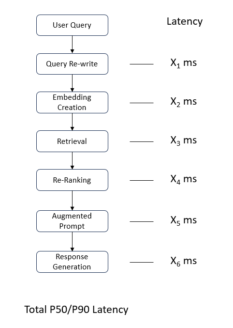
Also, most of the techniques mentioned for cost optimization also help directly in improving latency of the system like smaller models, optimized prompts, quantization etc.

There are also some additional latency specific optimization techniques which may prove to be beneficial for certain large-scale use cases -

1. Using a small Router LLM to first determine if Retrieval is required or is query can be answered directly by the LLM model itself. And if Retrieval is required, then it can also determine complexity of the query so as to route to bigger or smaller LLMs for response generation.

2. Keep frequently submitted prompts and their responses in cache memory. Here, first match incoming query with previously answered query and if match is found, send cache content to a smaller LLM for response generation. Use the typical flow only if there is no match found cache.

Note: Caching requires careful invalidation when source documents or permissions change.

Evaluation

AI-based systems require extensive evaluation as it is the single most important component which can help ensure if the system will fail in Production or not.

Generally in Production RAG Systems, evaluation is done in 2 Stages -

1. Retrieval Evaluation

2. Generation/RAG Evaluation

Retrieval Evaluation

Are we retrieving the right information ?

There are some standard evaluation metrics widely used to measure retrieval accuracy -

$$Precision @ K = \frac {Number\ of\ relevant\ documents\ in\ K} {K}$$

$$ Recall @ K = \frac {Number\ of\ relevant\ documents\ in\ K} {Total\ Relevant\ Documents}$$

$$ MeanAveragePrecision\ (MAP) = Average\ [\frac {1}{|Q|}\sum_{q\in Q} AP(q)]$$

$$ AveragePrecision(q) = \frac {1}{R_q}\sum_{k=1}^K Precision@k\ *\ rel_k$$

$$ MeanReciprocalRank\ (MRR) = \frac {1}{|Q|}\sum_{i=1}^{|Q|} \frac {1}{Rank_i}$$

$$ NormalizedDiscountedCumulativeGain (NDCG@K) = \frac {DCG@K}{IDCG@K}$$

$$ DCG@K = \sum_{i=1}^K \frac {rel_i}{log_2(i+1)}$$

$$rel_i = relevant\ score\ of\ item\ at\ position\ i$$

$$ IDCG@K = Max\ DCG\ score.\ Calculated\ by\ sorting\ all\ items\ by\ relevance\ in\ descending\ order$$

Where,

R_q = number of relevant items for query q; Q = collection of total queries

Generation/RAG Evaluation

Given the retrieved context, did the system generate a good answer?

Here, I will mention two most common RAG evaluation techniques used in Production -

1. Human-as-a-Judge - AI Engineers curate a large set of prompts covering as much diversity as possible including document-related prompts to evaluate relevance accuracy as well as other prompts to evaluate guardrails and security. Each one of the prompts is then manually evaluated by humans for pre-decided criteria

2. LLM-as-a-Judge - Most of the time AI systems are first evaluated by another LLM(s) which act a Judge against a pre-decided rubric of evaluation criteria. 'RAGAS' is one such library which provides this functionality. Here, the rubric generally comprises of metrics like -

   1. Response Relevancy - Evaluates relevance of response regardless of factual accuracy. Here input prompt is compared, in terms of similarity, with synthetic prompts which could have led to the same response.

   2. Faithfulness - It determines factual accuracy by making additional LLM calls to determine if the response claim is factually supported by the retrieved information.

   3. Correctness - When an Expected/Reference Answer exists, it determines if the answer matches the same.

There are also additional metrics like Noise Sensitivity and Citation Ability which are sometimes used to evaluate effectiveness of the RAG system.

Tip: RAGAS is a great library for RAG evaluation. Reading about certain metrics and definitions (not just their implementation) brings better clarity on applicability of certain metrics for robustness of your specific use case.

Before we end this article, I wanted to share my personal thoughts on debugging RAG Pipelines.

Debugging

Understanding points of failure in a Production RAG Pipeline and their possible reasons is one of the most underrated skill in my opinion. If mapped well, this can save a lot of valuable engineering time and also help maintain user trust.

Some of the most common failure nodes in a RAG system and their potential causes are -

Failure Mode	Source of Problem
Relevant document isn't retrieved	Retrieval
Relevant document is retrieved but buried at rank 20	Re-Ranking
Correct document retrieved but chunk lacks context	Chunking
Correct context retrieved but LLM ignores it	Generation/Prompt
Correct answer but unacceptable latency/cost	System Design

---

That's all on RAG for now. Feel free to comment below if there are some other possibilities in the architecture or optimization or evaluation which helped you improve your specific use cases.